Sankey diagram

Sankey diagram

.

Sankey diagrams are well-suited to visualize flows of differential expression genes ( anything is also ) and with different categories or types.

.

input data
divide DEGs into three groups : with SXL，with MSL2 and with SXL.MSL2

# ------ input data

# MSL-2 binding in genes (+150 bp)
setwd("E:/220625_PC/R workplace/220320_SXL/240808_msl2_peak.in_gene_S2/")
# msl2_in_genes <- read.table("peak_in_gene.500bp.txt",header = F)
msl2_in_genes <- read.table("peak_in_gene.150bp.txt",header = F)
head(msl2_in_genes)
msl2_in_genes <- msl2_in_genes[,-c(16,18)]
colnames(msl2_in_genes) <- c("chr","start","end","peak_name","score","strand","foldchange","-log10 pvalue",
                             "-log10 qvalue","summit_position",
                             "g.chr","g.start",".g.end","g.strand","geneID","gene_name")
msl2_in_genes_filter <- subset(msl2_in_genes, grepl("FBgn", msl2_in_genes$geneID))

msl2_in_genes_filter <- msl2_in_genes_filter[msl2_in_genes_filter$score >200 & 
                                               msl2_in_genes_filter$foldchange > 2,]
msl2_in_genes_gene <- msl2_in_genes_filter[!duplicated(msl2_in_genes_filter$geneID),]


# Sxl.peak
setwd("E:/220625_PC/R workplace/220320_SXL/Fan.data/sxl_peak_bind_DEGs/20220328/")
peak_intersect_feature <- read.table("Sxl-bind-feature.txt",header = F)
head(peak_intersect_feature)
colnames(peak_intersect_feature) <- c("peak.chr","peak.strat","peak.end","peak.xuhao","log10Pv","peak.strand","siteScore","V8",
                                      "chr","start","end","V12","ID_feature","strand")
peak_feature <- peak_intersect_feature
library(stringr)
peak_feature$GeneID <- str_split(peak_feature$ID_feature,"\\_",simplify = T)[,1]
peak_feature$transID <- str_split(peak_feature$ID_feature,"\\_",simplify = T)[,2]
peak_feature$feature <- str_split(peak_feature$ID_feature,"\\_",simplify = T)[,3]

peak_feature <- peak_feature[peak_feature$strand == peak_feature$peak.strand,]
length(unique(peak_feature$GeneID)) # peak in 5167 genes
length(unique(peak_feature$peak.xuhao)) # total

peak_SXL_genes <- peak_feature[!duplicated(peak_feature$GeneID),]
  

# DEGs 
setwd("E:/220625_PC/R workplace/220320_SXL/220421_SXL.S2/DEGs/")
S2_up <- read.csv("diff_gene_up.csv",header = T,row.names = 1)
S2_down <- read.csv("diff_gene_down.csv",header = T,row.names = 1)

.

plot

# ------ sankey 

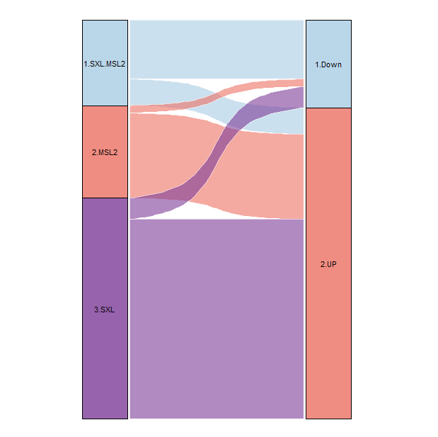
S2_DEG <- rbind(S2_up[,c(1,3)],S2_down[,c(1,3)])
S2_DEG$S2.TYPE <- ifelse(S2_DEG$GeneID %in% msl2_in_genes_gene$geneID & 
                           S2_DEG$GeneID %in% peak_SXL_genes$GeneID, "1.SXL.MSL2",
                         ifelse(S2_DEG$GeneID %in% msl2_in_genes_gene$geneID,"2.MSL2",
                                ifelse(S2_DEG$GeneID %in% peak_SXL_genes$GeneID,"3.SXL","4.non"))) %>% as.factor()
S2_DEG$DEG <- ifelse(S2_DEG$GeneID %in% S2_up$GeneID ,"2.UP","1.Down") %>% as.factor()

S2_DEG <- S2_DEG[!S2_DEG$S2.TYPE == "4.non",]
test_S2_UP <- S2_DEG[S2_DEG$DEG == "2.UP",]
test_S2_Down <- S2_DEG[S2_DEG$DEG == "1.Down",]


library(ggalluvial)
rownames(S2_DEG) <- S2_DEG$GeneID
S2_DEG <- S2_DEG[,c(-1,-2)]
S2_DEG$ID <-  paste0(S2_DEG$S2.TYPE,"_",S2_DEG$DEG)

plot_dat <- as.data.frame(table(S2_DEG$ID))
colnames(plot_dat) <- c("ID","num")

plot_dat$S2.TYPE <- str_split(plot_dat$ID,"\\_",simplify = T)[,1]
plot_dat$DEG <- str_split(plot_dat$ID,"\\_",simplify = T)[,2]
rownames(plot_dat) <- plot_dat$ID
plot_dat <- subset(plot_dat,select=c("S2.TYPE","DEG","num"))

library(ggalluvial)
plot_dat$S2.TYPE <- factor(plot_dat$S2.TYPE,
                           levels = c("1.SXL.MSL2","2.MSL2","3.SXL"))

df <- to_lodes_form(plot_dat,
                    key = "x", value = "stratum", id = "alluvium",
                    axes = 1:2)

col <- c("#A9CCE3","#EC7063","#7D3C98",
         "#A9CCE3","#EC7063","#7D3C98",
         "#A9CCE3","#EC7063","#7D3C98")

setwd("E:/220625_PC/R workplace/220320_SXL/202404_Fig/241106/")
pdf("sankey_S2_only.pdf",width = 7,height = 6)
ggplot(df, aes(x = x, y=num, fill=stratum, label=stratum,
               stratum = stratum, alluvium  = alluvium))+ # input data
  geom_flow(width = 0.22, # Line width
            curve_type = "arctangent",#Curve shapes: linear、cubic、quintic、sine、arctangent、sigmoid
            alpha = 0.6, 
            color = "white")+ # the color of intervals
  geom_stratum(width = 0.20, alpha=0.8)+ # The width and transparency of the rectangle in the image
  geom_text(stat = 'stratum', size = 3, color = 'black')+
  scale_fill_manual(values = col)+ #  Color
  theme_void()+ # Theme (without axes or grid lines)
  theme(legend.position = 'none') # Remove the legend
dev.off()

.