1
2
3
4
5
6
7
8
9
10
11
12
13
14
15
16
17
18
19
20
21
22
23
24
25
26
27
28
29
30
31
32
33
34
35
36
37
38
39
40
41
42
43
44
45
46
47
48
49
50
51
52
53
54
55
56
57
58
59
60
61
62
63
64
65
66
67
68
69
70
71
72
73
74
75
76
77
78
79
80
81
82
83
84
85
86
87
88
89
90
91
92
93
94
95
96
97
98
99
100
101
102
103
104
105
106
107
108
109
110
111
112
113
114
115
116
117
118
119
120
121
122
123
124
125
126
127
128
|
setwd("E:/220625_PC/R workplace/220801_peak_density/")
colnames(cvgList)
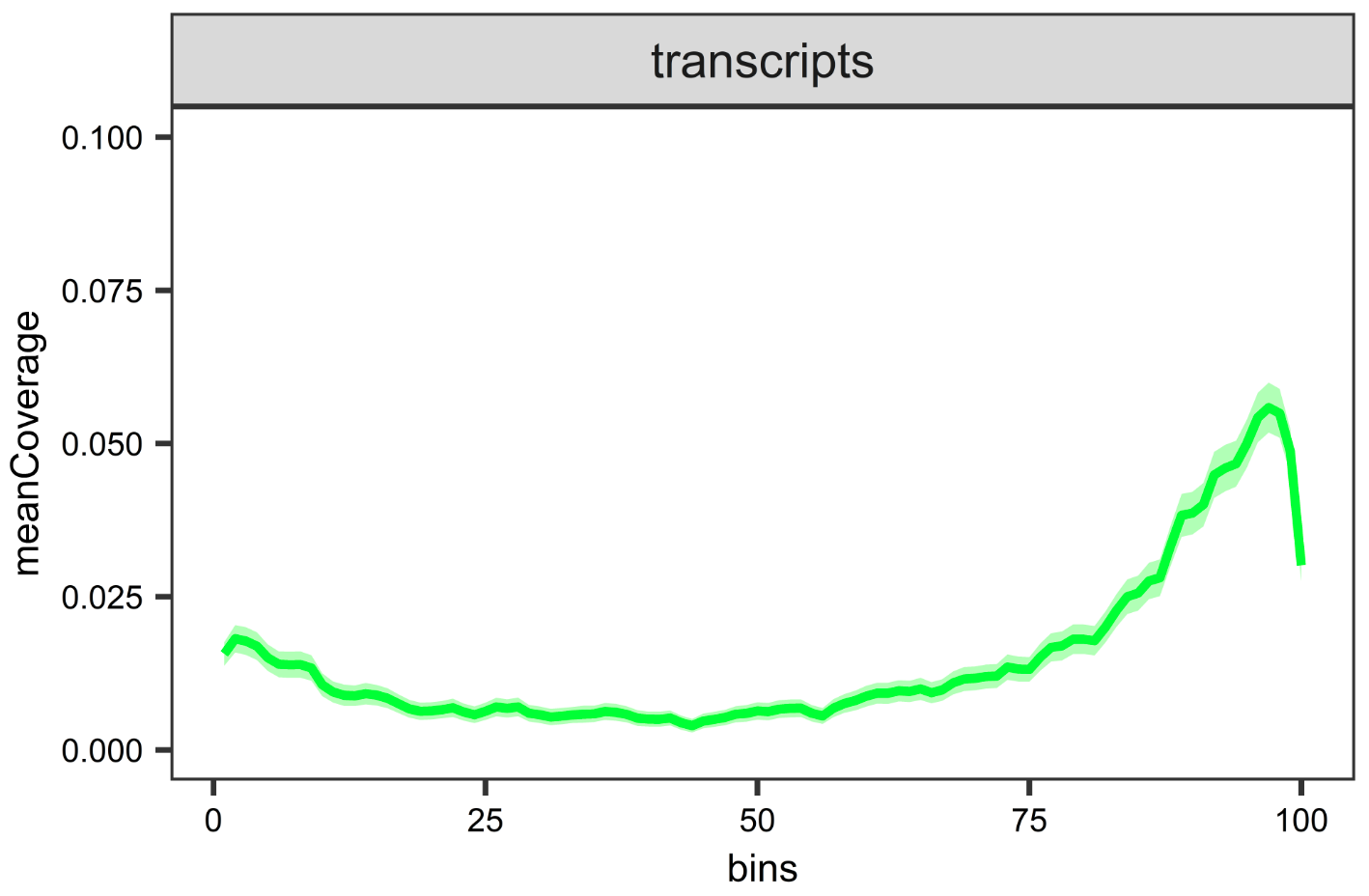
tiff("Transcripts-coverage.tiff",units = "in",width = 9,height = 9,res = 900)
list_Transcripts <- cvgList[cvgList$feature=="transcripts",]
ggplot2::ggplot(list_Transcripts, aes(x = bins, y = meanCoverage)) +
geom_ribbon(fill = 'green', alpha=0.3,
aes(ymin = meanCoverage - standardError * 1.96,
ymax = meanCoverage + standardError * 1.96)) +
geom_line(color = 'green',size=2) + theme_bw(base_size = 28) +
facet_wrap( ~ feature,ncol = 1) +
ylim(0,0.1)+
theme(panel.grid =element_blank(),
panel.grid.major = element_blank(),
panel.grid.minor = element_blank())+
theme(axis.text.x = element_text(size = 15,color = "black"),
axis.text.y = element_text(size = 15,color = "black"),
axis.title.x = element_text(size = 18,color = "black"),
axis.title.y = element_text(size = 18,color = "black"))
dev.off()
setwd("E:/220625_PC/R workplace/220801_peak_density/")
colnames(cvgList)
tiff("3UTR-1.tiff",units = "in",width = 9,height = 9,res = 900)
list_3UTR <- cvgList[cvgList$feature=="threeUTRs",]
ggplot2::ggplot(list_3UTR, aes(x = bins, y = meanCoverage)) +
geom_ribbon(fill = 'blue', alpha=0.3,
aes(ymin = meanCoverage - standardError * 1.96,
ymax = meanCoverage + standardError * 1.96)) +
geom_line(color = 'blue',size=2) + theme_bw(base_size = 28) +
facet_wrap( ~ feature,ncol = 1) +
ylim(0,0.1)+
theme(panel.grid =element_blank(),
panel.grid.major = element_blank(),
panel.grid.minor = element_blank())+
theme(axis.text.x = element_text(size = 15,color = "black"),
axis.text.y = element_text(size = 15,color = "black"),
axis.title.x = element_text(size = 18,color = "black"),
axis.title.y = element_text(size = 18,color = "black"))
dev.off()
setwd("E:/220625_PC/R workplace/220801_peak_density/")
colnames(cvgList)
tiff("5UTR-1.tiff",units = "in",width = 9,height = 9,res = 900)
list_5UTR <- cvgList[cvgList$feature=="fiveUTRs",]
ggplot2::ggplot(list_5UTR, aes(x = bins, y = meanCoverage)) +
geom_ribbon(fill = 'blue', alpha=0.3,
aes(ymin = meanCoverage - standardError * 1.96,
ymax = meanCoverage + standardError * 1.96)) +
geom_line(color = 'blue',size=2) + theme_bw(base_size = 28) +
facet_wrap( ~ feature, ncol = 1) +
ylim(0,0.1)+
theme(panel.grid =element_blank(),
panel.grid.major = element_blank(),
panel.grid.minor = element_blank())+
theme(axis.text.x = element_text(size = 15,color = "black"),
axis.text.y = element_text(size = 15,color = "black"),
axis.title.x = element_text(size = 18,color = "black"),
axis.title.y = element_text(size = 18,color = "black"))
dev.off()
setwd("E:/220625_PC/R workplace/220801_peak_density/")
colnames(cvgList)
tiff("CDS-1.tiff",units = "in",width = 9,height = 9,res = 900)
list_CDS <- cvgList[cvgList$feature=="cds",]
ggplot2::ggplot(list_CDS, aes(x = bins, y = meanCoverage)) +
geom_ribbon(fill = 'blue', alpha=0.3,
aes(ymin = meanCoverage - standardError * 1.96,
ymax = meanCoverage + standardError * 1.96)) +
geom_line(color = 'blue',size=2) + theme_bw(base_size = 28) +
facet_wrap( ~ feature, ncol = 1) +
ylim(0,0.1)+
theme(panel.grid =element_blank(),
panel.grid.major = element_blank(),
panel.grid.minor = element_blank())+
theme(axis.text.x = element_text(size = 15,color = "black"),
axis.text.y = element_text(size = 15,color = "black"),
axis.title.x = element_text(size = 18,color = "black"),
axis.title.y = element_text(size = 18,color = "black"))
dev.off()
setwd("E:/220625_PC/R workplace/220801_peak_density/")
colnames(cvgList)
tiff("Intron-2.tiff",units = "in",width = 9,height = 9,res = 900)
list_Intron <- cvgList[cvgList$feature=="introns",]
ggplot2::ggplot(list_Intron, aes(x = bins, y = meanCoverage)) +
geom_ribbon(fill = 'red', alpha=0.3,
aes(ymin = meanCoverage - standardError * 1.96,
ymax = meanCoverage + standardError * 1.96)) +
geom_line(color = 'red',size=2) + theme_bw(base_size = 28) +
facet_wrap( ~ feature, ncol = 1) +
ylim(0,0.1)+
theme(panel.grid =element_blank(),
panel.grid.major = element_blank(),
panel.grid.minor = element_blank())+
theme(axis.text.x = element_text(size = 15,color = "black"),
axis.text.y = element_text(size = 15,color = "black"),
axis.title.x = element_text(size = 18,color = "black"),
axis.title.y = element_text(size = 18,color = "black"))
dev.off()
setwd("E:/220625_PC/R workplace/220801_peak_density/")
colnames(cvgList)
tiff("Exon-2.tiff",units = "in",width = 9,height = 9,res = 900)
list_Exon <- cvgList[cvgList$feature=="exons",]
ggplot2::ggplot(list_Exon, aes(x = bins, y = meanCoverage)) +
geom_ribbon(fill = 'red', alpha=0.3,
aes(ymin = meanCoverage - standardError * 1.96,
ymax = meanCoverage + standardError * 1.96)) +
geom_line(color = 'red',size=2) + theme_bw(base_size = 28) +
facet_wrap( ~ feature, ncol = 3) +
ylim(0,0.1)+
theme(panel.grid =element_blank(),
panel.grid.major = element_blank(),
panel.grid.minor = element_blank())+
theme(axis.text.x = element_text(size = 15,color = "black"),
axis.text.y = element_text(size = 15,color = "black"),
axis.title.x = element_text(size = 18,color = "black"),
axis.title.y = element_text(size = 18,color = "black"))
dev.off()
|